The IS Curve and Aggregate Demand
Week 04
1. The Components of Aggregate Expenditure
The Aggregate Demand for G&S
At the level of the entire economy, there are two sides in the market for Goods & Services (G&S):
- The Demand side: G&S are demanded, which is translated into a a set of “Planned Expenditures”
- The Supply side : G&S are produced/supplied at a certain market price.
The Aggregate Demand for G&S
. . .
The total amount of planned expenditures on G&S, which we will call by aggregate demand \((D)\) is given by: 1
\[D=C+I+G+NX \tag{1}\]
- \(C\): Personal consumption expenditures on G&S
- \(I\): Investment expenditures on G&S
- \(G\): Government purchases of G&S
- \(NX\): Net exports of G&S
Personal Consumption Expenditures
. . .
In a developed market economy, personal consumption expenditures \(C\) are explained by three fundamental variables:2
\[ C=\overline{C}+c \cdot \underbrace{(Y-T)}_{=Y_D}-b \cdot r \tag{2} \]
- \(\overline{C}\) : exogenous consumption expenditures
- \(Y\) : GDP, income, or “output”
- \(T\) : income taxes
- \(Y_D\) : disposable income
- \(r\) : real interest rate
- \(c>0\) : parameter (known as the “marginal propensity to consume”)
- \(b>0\) : parameter
Investment Expenditures
In a developed market economy, the level of investment depends upon:
- \(\overline{I}\) : exogenous investment (the textbook calls it “Autonomous” investment)
- \(r_i\) : real interest rate charged on investments
Banks charge \(r_i\) as the sum of the risk-free market real interest rate \((r)\) and the risk-premium or spread \((\overline{f})\):3 \[r_i=r+\overline{f} \tag{3}\]
Therefore, the demand expenditures on investment G&S will be given by: \[I=\overline{I}-d \cdot\underbrace{(r+\overline{f})}_{r_i} \tag{4}\]
- where \(d\) is a parameter: (\(d>0\))
Financial Frictions and Investment
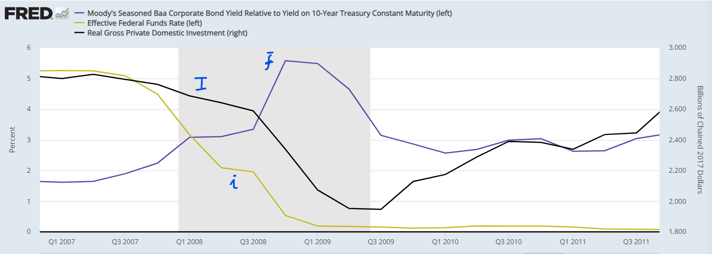
In the great financial crisis of 2007-2010, the inverse relationship between \((\overline{f})\) and \(I\) can be easily spotted in the figure below: \(\uparrow \overline{f}, \downarrow I\), despite \((i)\) going down. And \(\downarrow \overline{f}, \uparrow I\), despite \(i\) remaining at \(0 \%\).
Government Expenditures and Income Taxes
- The level of government expenditures on G&S is a result of a political decision in the Parliament
- So \((G)\) is exogenously determined: \[ G=\overline{G} \tag{5} \]
Government Expenditures and Income Taxes
The level of income taxes \((T)\) increases with income, so we could describe taxes with the following tax function: \[ T=\overline{T}+t \cdot Y \tag{6} \] where \(t\) is the marginal income tax rate.
However, for simplicity, we will assume that the level of income taxes is also exogenously determined: \[ T=\overline{T} \tag{7} \]
This simplification will not significantly change our results in this course.
Net-Exports Expenditures
Net-exports expenditures are made up of two components:
Autonomous net exports \((\overline{N X})\)
Net exports affected by changes in real interest rates \((r)\)
Putting together these two components, we get: \[ N X=\overline{N X}-x \cdot r \tag{8} \] where \(x>0\) is a parameter.
Why are net exports negatively dependent on the real interest rate?
See next slide.
Why \(r\) Affects Net-Exports?
An example. Suppose the ECB (European Central Bank) reduces interest rates in the EuroZone (EZ): \[ \downarrow r_{_{(EZ)}} \]
- This leads to financial investments denominated in € becoming less internationally attractive: they now have a lower return.
- Lower demand for € in the foreign exchange markets, leads to a depreciation of the € against other currencies.
- A depreciated € leads to G&S produced in the EuroZone becoming relatively less expensive than before, resulting in an increase in NX from Euro countries.
- So: \(\qquad \downarrow r \Rightarrow \text { national currency depreciates } \Rightarrow \uparrow N X\)
2. The IS Curve
The Relationship Betwwen GDP and Demand
. . .
From eq. (1), we saw that the level of aggregate demand is given by:
\[D=C+I+G+NX\]
. . .
And from week 2, we know that GDP \((Y)\) can be calculated by the sum of all expenditures on final G&S. So we must have:
\[Y=D \tag{9}\]
. . .
Therefore, we can relate GDP with the demand side by writing:
\[Y=C+I+G+NX \tag{10}\]
Eq. (10) allows us to obtain a very simple and useful curve: IS curve
Derivation of the IS Curve
To obtain an equation that reflects the impact of demand forces on the level of GDP \((Y)\), we have to do as follows:
. . .
\[Y=C+I+G+NX\]
. . .
\[ Y=\underbrace{\overline{C}+c \cdot(Y-\overline{T})-b \cdot r}_{=C}+\underbrace{\overline{I}-d \cdot(r+\overline{f})}_{=I}+\underbrace{\overline{G}}_{=G}+\underbrace{\overline{NX}-x \cdot r}_{=NX} \]
. . .
Rearranging better the previous equation, we get:
\[ Y=\overline{C}+\overline{I}-d \cdot \overline{f}+\overline{G}+\overline{N X}-c \cdot \overline{T}+c \cdot Y-(b+d+x) \cdot r \tag{11} \]
. . .
Smplify the exposition, by grouping together all the elements with an over bar, and call it the Exogenous/Autonomous Aggregate Demand:
\[ \overline{A}=\overline{C}+\overline{I}-d \cdot \overline{f}+\overline{G}+\overline{N X}-c \cdot \overline{T} \tag{12} \]
Derivation of the IS Curve (continuation)
Inserting eq. (12) into eq. (11), we get a very simple equation: \[ Y=\overline{A}+c \cdot Y-(b+d+x) \cdot r \]
. . .
which can be solved for \(Y\) as follows:
\[ Y=\frac{1}{1-c} \cdot \overline{A}-\frac{(b+d+x)}{1-c} \cdot r \tag{13} \]
. . .
But we can simplify it even further:
\[ Y=m \cdot \overline{A}-m \cdot \phi \cdot r \tag{14} \]
- \(\frac{1}{1-c}=m \quad \longrightarrow\) \(m\) is a parameter know as the demand multiplier
- \(b+d+x=\phi \quad \longrightarrow\) \(\phi\) is a parameter (or a sum of parameters)
The IS Curve: Summary
For the set of parameters \(\{m,\phi\}\), the level of Aggregate Demand and GDP \((D, Y)\) is positively affected by the level of the autonomous/exogenous aggregate demand \((\overline{A})\), and negatively by the level of the real interest rate \((r)\) : \[ Y=m \cdot \overline{A}-m \cdot \phi \cdot r \tag{14'} \]
. . .
- Notice that, to simplify things, we have defined:
- \(m=\frac{1}{1-c}>1\)
- \(\phi=b+d+x>0\)
- \(\overline{A}=\overline{C}+\overline{I}-d \cdot \overline{f}+\overline{G}+\overline{N X}-c \cdot \overline{T}\)
IS Curve: Graphical Representation
For a given level of \((\overline{A})\), an increase in \((r)\) will cause a reduction in aggregate demand \((D)\), which will lead to a decline in GDP \((Y)\), and vice-versa. 
IS Curve: Graphical Representation
- \(\Delta r=+2pp\)
- \(\Delta \overline{A}=0\)
- \(\Delta Y=-2 trillion\)
- If \(\Delta \overline{A} \neq 0\), the IS would shift to the right/left
3. Forces that Shift the IS Curve
Exogenous Demand and Shifts in the IS Curve
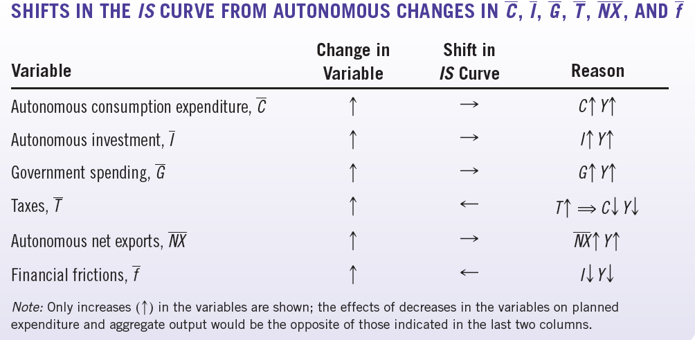
Recall that the exogenous/autonomous aggregate demand is given by:4 \[ \overline{A}=\overline{C}+\overline{I}-d \cdot \overline{f}+\overline{G}+\overline{N X}-c \cdot \overline{T} \]
A change in any of these components of \(\overline{A}\) will force the IS curve to shift.
For example, consider an increase in public spending: \(\Delta \overline{G}>0\). From the expression above we get:
\[\Delta \overline{A}=\Delta \overline{G}>0\]However, from the IS curve we know that: \[ \Delta Y=m \cdot \Delta \overline{A} \quad \Longrightarrow \quad \Delta Y=m \cdot \Delta \overline{G} \]
Because \(m>1\), we have: \(\uparrow \overline{G} \Rightarrow \uparrow \overline{A} \Rightarrow \uparrow Y\) : the IS curve shifts to the right
Another Example of a Shift in the IS Curve
The exogenous aggregate demand:\(\ \ \overline{A}=\overline{C}+\overline{I}-d \cdot \overline{f}+\overline{G}+\overline{N X}-c \cdot \overline{T}\)
A change in the spread (or as the textbook calls it: the “financial friction”) will also shift the IS curve. Suppose that the spread increases by \(4\) percentage points: \[\Delta \overline{f}=+4pp\]
From the exogenous aggregate demand expression above we get:
\[\Delta \overline{A}= - d \cdot \Delta \overline{f}= - d \times 4pp\]However, from the IS curve we know that: \[ \Delta Y=m \cdot \Delta \overline{A} \quad \Longrightarrow \ \Delta Y= m \cdot ( -d \times 4pp) \]
Because \(m>1, d>0\), we have: \(\uparrow \overline{f} \Rightarrow \downarrow \overline{A} \Rightarrow \downarrow Y\) : the IS curve shifts to the left
A Shift in the IS: a Graphical Example
If \(\uparrow \overline{G} \ \Rightarrow \ \uparrow \ \overline{A} \ \Rightarrow \ \uparrow Y\) , the IS shifts to the right:
. . .
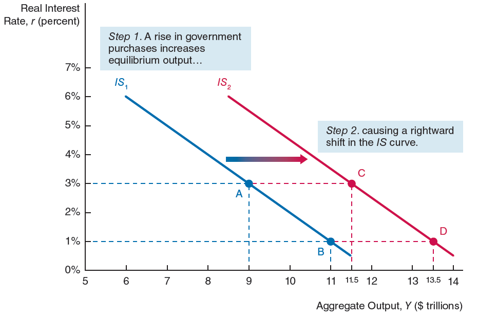
- The IS shifts to the right for any \(r\) level
- The shift is the same for \(r=3\%\), \(r=1\%\), \(r=0\%\) , or …
A Shift in the IS: another Graphical Example
If \(\uparrow \overline{T} \ \Rightarrow \ \downarrow \ \overline{A} \ \Rightarrow \ \downarrow Y\), the IS shifts to the left:
. . .
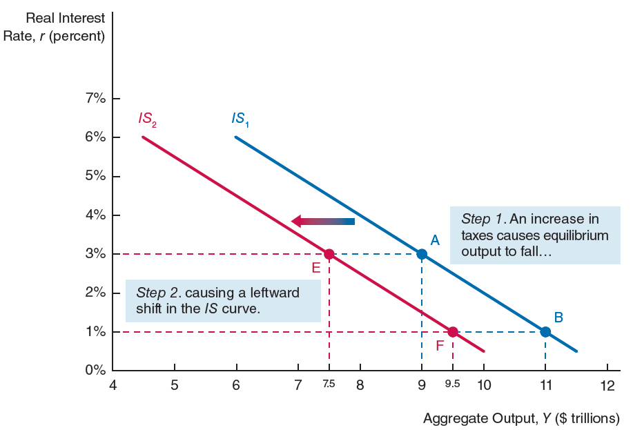
- The IS shifts to the left for any \(r\) level
- The shift is the same for \(r=3\%\), \(r=1\%\), \(r=0\%\) , or …
The Multiplier of Aggregate Demand
An increase/decrease in \(\overline{A}\), will shift the IS curve leading to an increase/decline in aggregate demand and GDP. But by how much?
It will depend upon the value of the demand multiplier \(m\) and the value of the shock.
As \(0<c<1\), then \[ m=\frac{1}{1-c}>1 \quad \Rightarrow \quad \Delta Y= m \cdot \Delta \overline{A} \quad \Rightarrow \quad {\color{blue} {\Delta Y > \Delta \overline{A}}} \]
Where \(\overline{A}=\overline{C}+\overline{I}-d \cdot \overline{f}+\overline{G}+\overline{N X}-c \cdot \overline{T}\)
One shock upon \(\overline{A}\) is amplified/multiplied through the other components of expenditure: the higher \(c\) is, the higher will be \(m\).
A Textbook Useful Table
Footnotes
The textbook uses \(Y^{pe}\) instead of \(D\). For simplicity we choose \(D\) for “demand”. The notation is better and it is more intuitive.↩︎
In eq. (2), where we use \(c\), the textbook uses \(mpc\), and where we have \(b\) the textbook uses \(c\). Our notation is easier to manage.↩︎
The textbook calls \(\overline{f}\) a financial friction. The three terms represent the same thing: a measure of risk.↩︎
No need to memorize this expression. Try to understand which ones have a negative/positive impact upon \(\overline{A}\).↩︎